*Disclaimer: This scenario is a case, all companies mentioned are based on fictional scenarios
Step 1: Business Understanding
The purpose of this section is to understand what the business problem and the stakeholders that will be understanding the work that I am performing. The stakeholder of my project is a real-estate consulting start-up that tries to help clients increase the value of their home. The main purpose of this algorithm is predictive, meaning that the model should be able to take in attributes of houses, and to predict price increases associated with it.
The secondary purpose of this algorithm is inferential, meaning that the model should reveal something about the relationship between the attributes of a housing attributes and its price. I will apply my knowledge of statistics to include appropriate dialogue about these relationships. This could help home-owners take the necessary steps to modify their home to maximize a potential return.
Step 2: Data Understanding
First, I inferred that the data comes from Kings County, Washington, based on what I can see from latitude and longitude. Second, it includes several items related to housing information, including beds and baths, lot size, and condition/grade. This data is useful because it has many attributes that can impact the target variable. In this case, I will be using price as my target variable and will use the other variables to predict price using regression.
Step 3: Data Preparation
In my data, I clean each column by checking for empty or missing data, remove outliers, and check for erroneous data from typos. This ensures that my models are getting proper data that allows for better results.
Step 4: Modeling
The first step in my modeling is to create a heatmap to get the most correlated variables. As you can see below, those variables were grade and sqft_living.
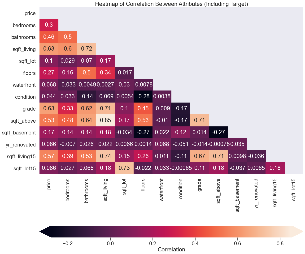
After removing highly variables for multicollinearity, I ran my baseline model. For both of my variables, I got a train score of .403 and a validation score of .400
Model 2.0
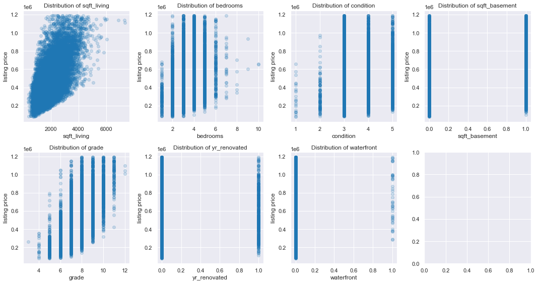
I then created a model based on all numeric features, including bedrooms, sqft_living, condition, and grade. This model generated a train score of .488 and a validation score of .485. It is getting better, but I think there is a better model.
Final Model
For this final model, I ran a for loop to generate every possible model for the 7 variables: floors, condition, sqft_basement (binary), waterfront, yr_renovated, sqft_living and grade. I generated 63 models and their related train/validation scores.
The model that got me the best scores had all 7 variables listed above, with a train score of .505 and a validation score of .498
After generating my final r^2 statistic I got .5166.
Step 5: Regression Results
To further understand my data and the results, I generated the following statistics:
-
For my mean absolute error, I got $118k, which implies that based on my mean house price of $481k, my model could be off by an absolute mean of $118k.
-
My coefficients for each variable are below. For every one increase in a related variable, the price should increase (decrease) by the following:
- Sq Feet Living Space: $98
- Bedrooms: -$17,333
- Condition: $45,169
- Basement: $38,708
- Grade: $88,275
- Renovated: $102,962
- Waterfront View: $242,268
As you can see, houses that have a waterfront or are renovated increase the price of a house greatly. As these are binary variables, they are not incremental. For each increase in grade, the house price goes up by $88k.
- Next, we check for normality to make sure our normality assumption is accurate. I generated a perfect fit line, as well as a Q-Q plot below.
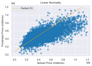
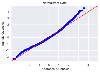
As you can see, the Q-Q plot is normal for most data, but trails off towards higher priced homes. Our line of fit seems to be linear, so no issues here, as well.
-
Next, is our variance inflation factor, to see how interrelated our features are. As you can see below, a lot of our variables are interrelated. This is to be expected, because the features of houses can be very correlated, for example, the more bedrooms there are in the house, the higher the sqft_living should be. To solve this issue, I am hoping to get more data in the future that shows more diverse features.
- sqft_living: 16.81
- bedrooms: 21.90
- condition: 20.35
- sqft_basement: 1.71
- grade: 38.24
- yr_renovated: 1.04
- waterfront: 1.01
-
Lastly, I check for homoscedasticity
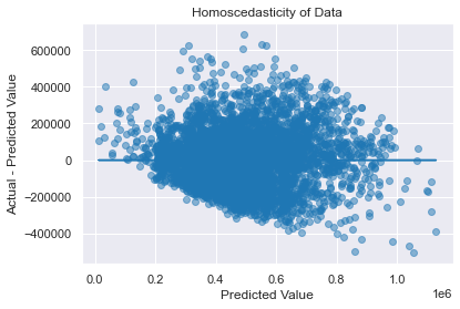
There doesn’t seem to be that bad of a funnel shape, there seems to be issues as the prices get larger, but hopefully we can sample a larger set of data with pricier houses to get a more accurate model in the future.
Next Steps
Our confidence in these coefficients should be not that high, as there seem to be some issues with the model. I hope to retest this model in the future with more data surrounding pricier houses, different features, such as location or color of house. I believe this added data should make our model stronger.